|
|
|
PLOTS AGAINST INFORMATION LAWS
Milan Kunz
Jurkovicova 13, 63800 Brno, Czech Republic
Received:
Abstract
Relations between the Zipf, Bradford and Lotka laws are shown to be different transformations of Ferrers graphs, which change their symmetries. Model distributions obtained on a logarithmic paper do not correlate with relations predicted by theoretitians. The three information laws are not precise inough, they are obsolete thumb rules, only.
-----------------------------------------------------------
Introduction
Extremely skewed distributions are basic distributions in the Nature: E.g. the distribution of bodies in the Universe according to their size, from microparticles till stars; the distribution of chemical elements from hydrogen till transuranium elements; the distribution of organisms, from one cell organisms till whales or sequoias. But nowhere they induced so many speculations as in information sciences.
Vlachy found in his bibliography published in the first number of Scientometrics [1] 437 items related to the Lotka law and similar phenomena. Since then the collection increased considerably.
Between papers dealing with so called information laws are many filled only with long series of mathematical formulas without any attempts to check the results otherwise than by mathematical sophistication.
It has been shown that the density of Lotka's own data did not meet requirements of his generalization [2] and Sichel [3] correlated different data satisfactorily by a three parametrical distribution. Despite it new specimens of speculations about specific properties of information distributions appear. On the recent Fourth International Conference on Bibliometrics, Informetrics and Scientometrics, September 11-15, 1993, Berlin 9 new contributions were presented [4-12].
It is difficult to disprove such subtle formal constructions theoretically. There is nothing wrong with them, excepts that they have nothing common with the physical reality.
The Bradford law can be valid only if the Lotka slope constant is 2 and the Zipf slope constant is 1. This relations are commonly accepted [13-18]. It is believed that the existence of three laws prescribes the asymptotic behavior of the distributions for ideal unlimited distributions. They should have infinite moments. The true problem of information distributions is that they have too low moments. Therefore they are assymetrical, truncated by the impossibility to realize negative frequencies or occurencies required to balance the distribution about the mean.
The arithmetical mean is usually too close to the lowest frequency and the median often coincide with it. Such problems appeared in quantum physics and can be compared e.g. with strange properties of helium near the absolute zero temperature. In physics any mathematical theory must explain observed facts, and this demand must be posed also on information laws. Some of such problems were discussed by Jones and Furnas [19].
In this paper we will study properties of real models of information laws. Any mathematical theory is good only if it corresponds to peculiarities of the described object. Because empirical information distributions are not reliable, it is necessary to replace them by ideal models, constructed as best possible approximations of studied laws. De Beaver remembered us that Price used logarithmic papers for preliminary correlations [20]. So we will do, too.
Matrices and Ferrers graphs
At first we will analyze graphically the process of collecting data in which three information laws are obtained. Each information item will be represented by one square of unit size. This is the first abstraction. It were better when the size corresponded to the length of a paper and the best if it could correspond to its importance, but such a sophistication should complicate our problem. We omit the process of collection of data and their classifications. It is indifferent, if squares represent items and columns words, as at Zipf, articles and journals, as at Bradford, or papers and authors, as at Lotka.
The information is embedded in the matrix and it has a matrix form, as on Fig. 1. In the original matrix A vectors are scattered accidentally. In B all items classified in columns are gathered. Formally, it is done by permutations of the rows of the matrix and matrices A and B are equivalent. In C the vectors are ordered in descending order according their size. It is again done by permutations of the rows and columns of the matrix. The contour describing the shape of ordered items (or its inner counterpart) is known as the Bradford law. The items in the matrix can be rearranged into a column diagram as on Fig. 1 D. It is done by multiplying the equivalent matrices by the unit vector column from the right.
In the number theory such diagrams are known as Ferrers graphs and are used as a tool to prove some theorems in the theory of partitions [21]. Perhaps we can use them to demonstrate relations between three information laws.
Suppose that we collected m items which are partitioned (classified) into n parts (vectors or otherwise named columns). This can be expressed as a summation equation
m = mj (1)
The index j is known as the rank and goes from 1 till n. In a partition parts of equal size k can exist and we can count their numbers nk which transforms the equation (1) as
m = nk mk (2)
Here we use for parts still the letter mk with the index k determining its size. The summation is made for index k going from 1 till m.
In the next step, without any modifications of the Ferrers graph (column diagram), we want to describe its contour (the shape of the outer edge of its area) by an analytical function. This gives us the third equation
mj = f(j) (3)
This equation corresponds to the Zipf law. The analytical function (3) should transform observed usually irregular shape of an column diagram into a straight line. This is possible, if we change linear scales of the Ferrers graph by another suitable scale, which weights index j or index k or both indices simultaneously. In other words, we change one linear scale or both of the graph by a suitable one, till the tops of columns appear on a straight line.
In the Bradford plot, the inner contour is the distorted baseline of the Zipf plot. Original columns appear between both contours as their difference. It means that the Bradford plot is a summation form of the Zipf plot or otherwise, the Zipf plot is a difference of the Bradford plot.
On Fig. 1.E an another arrangement of the items is shown. Here they are organized into columns according to their size.
On Fig. 1.F the difference of the Zipf plot according to the horizontal scale n is depicted which is simultaneously a difference of Fig. 1.E. Now the numbers nk of vectors having the length mk are counted on the horizontal scale . If they were normalized by dividing with their sum n, they determine the density of vectors in the multidimensional space. This is the Lotka plot. It appears to be a difference of the Zipf plot, but in statistics it is considered to be a basic distribution and on the Fig. 1.E the distribution of its sums is.
On Fig. 1 basic relations between three information laws are formulated without any ambiguities. Differences between them can not be in which field they are used, if in linguistics, scientometrics or bibliometrics, but only how good they are for describing observed data. They are different transformations of Ferrers graphs, which change their symmetries and answer different questions.
Ideal plots
The Lotka plots were used by Nicholls [22] for testing the Price square root law. But he was interested only in slope constants and neglected the possibility to check the validity of the Zipf and Bradford laws. The construction of model distributions is easy. We take the double logarithmic paper, choose the slope constant B and the initial point constant A, corresponding to the number of information vectors n1 with the occurency number m1 = 1, and find the nearest integer expected values nk at the integer values mk of the argument k. If one value is rounded down, the next value should be rounded up, to keep the correlation as close to the ideal line as possible.
On Fig. 2 is the Lotka plot for n = 100 and B = 2. There were neglected fractional expectations lower than 1. The highest mk = 10 and there are no gaps between highest frequencies. The Zipf projection of this best possible plot is on the Fig. 2, too, drawn with empty circles. The starting parameter C = 10. The parameter D can be estimated only for initial 6 points, the tail of the Zipf plot deviates considerably from linearity. The corresponding Bradford plot has no linear part at all.
On Fig. 3 is the Zipf plot for m1 = 100 (the number of papers of the most prolific author) and D = 1 and its Lotka projection. For n2 till n7 it were possible to use B = 2, but there remains a huge tail of values mk > 10 which deviation is opposite to observed deviations of empirical plots. The exact value n1 = 35 is too low, whereas n1 = 100 were acceptable for both plots. The Bradford plot is practically linear.
We left aside fractional expectations, where observed values must oscilate between zero and one, because information vectors are quantal phenomena. On Fig. 2, there should be occupied several positions in the range of frequencies 11-100, in 900 higher frequencies at least one, and so on. But such high frequencies do not usually occur in experimental sets of increased size.
It was already shown, that empirical data do not fit theoretical demands on relations between Lotka and Zipf laws [23], which were derived for infinite models. Real size distributions can not fulfill them.
Discussion
According to the Occam razor, no concept should be introduced, unless necessary. In our problem it is the notion of probability.
When a biologist is studying an organism or its part, he does not starts with contemplations, what the probability is, that such an organism exists or if the organism is homogeneous inough, that its one organ can represent the whole body. Statistics has important functions in our problem, but they are connected with tasks of stochastic sampling and comparing different sets of data and not with the existence of individual data sets.
Practically all scientometric and bibliometric data are collected for some systems corresponding e. g. to organisms. Three information laws have not validity of physical laws, as the gravitation law is, for example, but they are only empirical observations, as the Titius-Bode function is, correlating the distances of the Planets from the Sun. Accidentally, it can be formulated as log a = jlog1.85, where a is astronomical unit (the distance Earth-Sun) and j is the rank [24]. Different sets of data correspond to systems of planets at different stars. Our task is to find what they have common and to explain how differences are formed. Till now we can only tell that all observed systems are extremely skewed and this is not too much for so many studies.
Three information laws are thumb rules, only, and they can not be improved, because they do not describe observed facts satisfactorily. Because they are only different moments of one distribution, it is useless to test which from them gives a better fit in a given case. Their theory does not explain observed deviations from linearity of finite cases, where they are applied. They were usefull as simple tools of manual counts and for such purposes can be applied even now.
Deviations of plots empirical and modeled plots from linearity show, that two parametrical distributions are not able to describe observed information distributions exactly. It is necessary to improve the precision of the fit and measure it. Therefore, it were dumb to remain at three laws for evaluating computer data, or for comparing collections from different fields now, when more precise statistical evaluations could be made easy even for social scientists.
A standard program for linear regression gives for Lotka's data [25] the correlation coefficient -0.958345 and the standard deviation 148.4. The polynomial regression program gives for y = 1/(polynomial of 3. degree) the correlation coefficient 0.999867 and the standard deviation 8.47. For y = 1/(polynomial of 9. degree) the correlation coefficient was 0.999982 and the standard deviation 3.27.
But when all frequencies till 108 with zero occupancies were considered, the linear regression program was not able to calculate the Lotka function, the result was 99 orders out, but for y = 1/(polynomial of 9. degree) the correlation coefficient was 0.999887 and the standard deviation 6.15. I have already shown that the density of Lotka's data fails from linearity of his plot [2].
Basu [26] replaced tacitly the Bradford plot by another function. His attempt to derive the distribution is not convincing, but it gives a better fit and that is important.
This are real plots against the information laws. Today, it is possible to describe observed data with a much greater precision then with obsolete laws and old correlations will be outdated, soon.
It is time to awake from the dreams about simple information laws. Bad laws must be replaced even in information sciences. Using only mathematics, it were possible to prove that scientists are assymptotically vanishing structures.
Acknowledgement
I am indebted to Dr. J. Jelen from Research Institute of Macromolecular Chemistry, Brno, for the computer program Regrese.
References
1. Vlachy J.: Frequency distributions of scientific performance, Scientometrics, (1978) 109.
2. Kunz, M. Can the lognormal distribution be rehabilitated?
Scientometrics,1990, 18, 179.
3. Sichel H.S.: A bibliometric distribution which really works, Journal American Society Information Science, 31 (1980) 314.
4. Bookstein A.: Towards a multidisciplinary Bradford Law. Fourth International Conference on Bibliometrics, Informetrics and Scientometrics, September 11-15, 1993, Berlin, Book of Abstracts, Part I.
5. Eto H.: Bradford law, diffusion and spillover. Fourth International Conference on Bibliometrics, Informetrics and Scientometrics, September 11-15, 1993, Berlin, Book of Abstracts, Part I.
6. Karmeshu, Rao B.N., Krishnamachri A.: Bibliometric analysis - Applications of income inequality measurement techniques. Fourth International Conference on Bibliometrics, Informetrics and Scientometrics, September 11-15, 1993, Berlin, Book of Abstracts, Part I.
7. Morales M., Morales A.M.: Multidimensional selective rank method for a new holistic hierarchical ranking of scientific journals, Fourth International Conference on Bibliometrics, Informetrics and Scientometrics, September 11-15, 1993, Berlin, Book of Abstracts, Part II.
8. Nelson M.J.: Order statistics and the discrete Zipf-Lotka distribution, Fourth International Conference on Bibliometrics, Informetrics and Scientometrics, September 11-15, 1993, Berlin, Book of Abstracts, Part I.
9. Oluic-Vukovic V.: The meaning of Bradford's and Lotka's laws beyond their immediate context, Fourth International Conference on Bibliometrics, Informetrics and Scientometrics, September 11-15, 1993, Berlin, Book of Abstracts, Part II.
10. Sen S.K.: Understanding Zipfian phenomena, Fourth International Conference on Bibliometrics, Informetrics and Scientometrics, September 11-15, 1993, Berlin, Book of Abstracts, Part II.
11. Czervon H.J.: Time factor in bibliometric distributions: A comparative empirical study of two research specialties. Fourth International Conference on Bibliometrics, Informetrics and Scientometrics, September 11-15, 1993, Berlin, Book of Abstracts, Part I.
12. Sharada B.A.: Word frequency count in computational linguistics, Fourth International Conference on Bibliometrics, Informetrics and Scientometrics, September 11-15, 1993, Berlin, Book of Abstracts, Part II.
13. Haitun,S.D. Stationary Scientometric Distributions I: Different Approximations, Scientometrics, 4 (1982) 4, 525.
14. Yablonsky A.L.: Stable non-Gaussian distributions in scientometrics, Scientometrics, 7 (1985) 459.
15. Egghe L.: Consequences of Lotka's law for the law of Bradford, Journal of Documentation, 41 (1985) 173.
16. Chen Y.S., Leimkuhler F.F.: Analysis of Zipf's law: An index approach, Information Processing Management, 23 (1987) 171.
17. Glanzel W., Schubert A.: Price distribution. An exact formulation of Price's "square root law", Scientometrics, 7 (1985) 211.
18. Brookes B.C.: Towards informetrics: Haitun, Laplace, Zipf, Bradford and Alvey programme, Journal of Documentation, 40 (1984) 120.
19. Jones W.P., Furnas G.W.: Pictures of relevance: A geometric analysis of similarity measures, Journal American Society Information Science, 38 (1987) 420.
20. Beaver D. de B.: Lecture in memory of Derek de Solla Price, Fourth International Conference on Bibliometrics, Informetrics and Scientometrics, September 11-15, 1993, Berlin.
21. Andrews G.E.: The Theory of Partitions, Addison-Wesley, Reading, 1976.
22. Nicholls P.T.: Price's square root law: Empirical validity and relation to Lotka's law, Information Processing Management, 24 (1988) 171.
23. M.KUNZ, Lotka and Zipf: Paper dragons with fuzzy tails, Scientometrics, 13 (1988) 2289.
24. Vanysek V.: Zaklady astronomie a astrofyziky, Academia, Praha, 1980, p. 522.
25. Lotka A.: The frequency distribution of scientific productivity, Journal Washington Academy Sciences, 16 (1926) 317.
26. Basu A.: Hiearchical distributions and Bradford's law, Journal American Society Information Science, 43 (1992) 494.
Description of Figures:
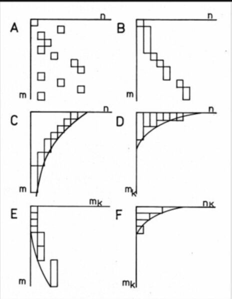
Fig. 1. Column diagrams of three information laws.
The description is in the text.
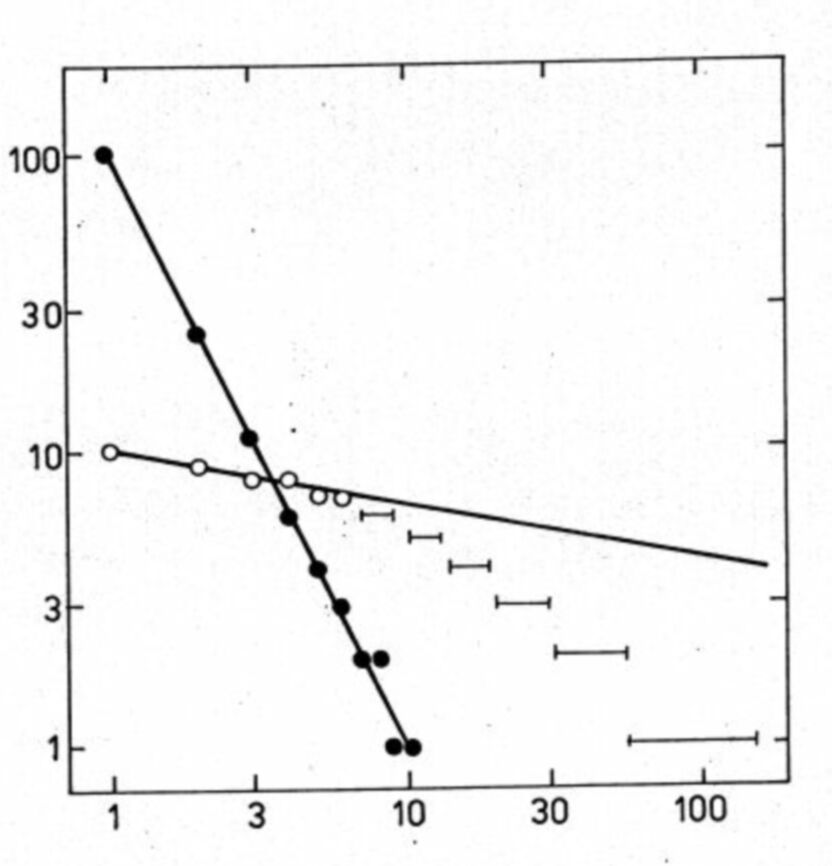
Fig. 2. Lotka plot and its Zipf projection.
Full circles are best possible values of the Lotka distribution of the given size. Empty circles show the Zipf plot of such data. The plot deviates from linearity considerably.
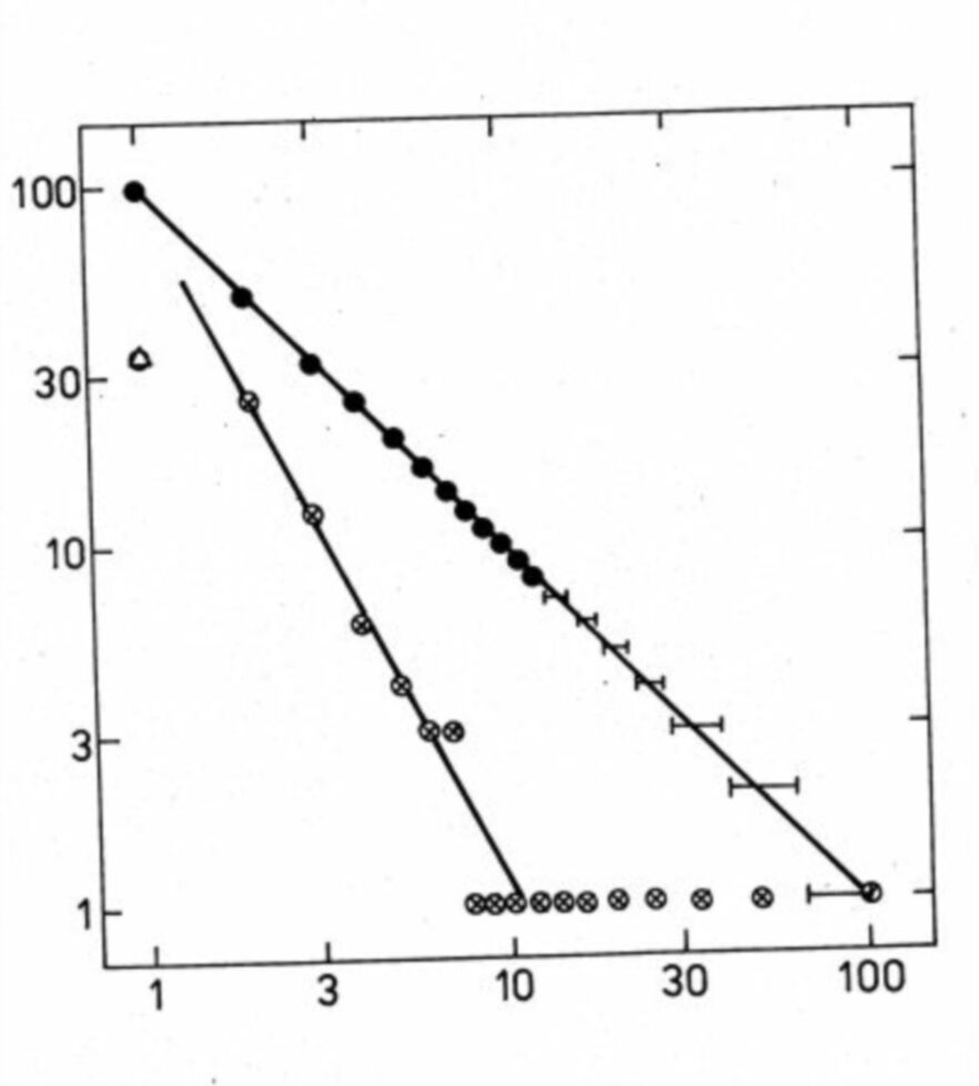
Fig. 3. Zipf plot and its Lotka projection.
Full circles are best possible values of the Zipf distribution of the given size. Empty circles show the Lotka plot of such data. The plot has only a limited linear part.